As machine learning models are increasingly used in applications such as hiring, lending, and other domains where decisions can have significant real-world impacts on people, it becomes paramount to ensure that these models are fair and unbiased. The use of fairness metrics can evaluate the impact of a model’s predictions towards different groups of individuals and help us address any potential biases, particularly those extracted from historical data. Thus, we can ensure that the model performs as intended, without bias in areas such as race, gender, age or other areas.

For example, a model trained on a dataset of historical hiring decisions may learn to prefer candidates who share the same demographic characteristics as previous hires, even if those characteristics are not relevant to the job requirements of the new role. This can perpetuate existing discrimination and result in a less diverse and inclusive workforce. To ensure fairness and prevent bias, we must work in a preventative manner and constantly monitor our data and models to take appropriate actions and ensure that the model’s decisions are equitable across different groups.

Below we show how to use our VIANOPS monitoring and observability platform in an easy way to both 1) compute fairness metrics between groups and 2) detect shifts in the data.

While bias and fairness in machine learning are two very correlated terms, these have subtle differences:

• • Bias: bias in machine learning models refers to the systematic prediction error towards a group of individuals. This can be caused when the group is underrepresented in the dataset, i.e. we trained the model on data that was lacking in diversity. Some of the issues that biased models can pose include (1) perpetuating and exacerbating unfairness towards minorities (2) giving inaccurate results (3) eroding trust and transparency in the institutions that use them, and/or (4) introducing legal and ethical implications.
  • Fairness: fairness aims to ensure that all predictions or decisions are not systematically biased against any group of individuals, meaning that the model should perform equally well across all the groups regardless of factors such as race or gender.

While both concepts are interrelated, when bias happens, it corresponds to being an issue with the accuracy of the model’s predictions only towards certain groups of individuals, while fairness is an issue with the ethical implications and societal impact of the model’s predictions.

The UCI Adult dataset¹ is a popular dataset which contains information on 32,000 individuals from the 1994 US Census database with features such as age, education level, marital status, occupation, and income. The dataset has a total of 48,842 instances and 14 attributes, which are a mix of both categorical and continuous variables. The target variable for this dataset is the income of the individual, which is classified into two classes: those earning over $50K per year and those earning less than $50K per year making it a binary classification problem. This dataset contains demographic and employment information about individuals, including their age, gender, race, and education level. These variables, used to predict the individual’s income level, can be a critical decision factor for various applications such as loan approval, job opportunities, and marketing. Therefore, using this dataset for machine learning algorithms without considering fairness metrics can lead to biased predictions.

Models that are trained on such datasets, can achieve high accuracy scores, but this may not reflect their performance in real-world scenarios if the data has bias or the distribution changes with time. Models will learn to make predictions based on the biases present in the training data, leading to unfair decisions that perpetuate biases and inequality, thereby creating systems of bias and inequality. The challenge is that these biases can be subtle and difficult to identify and simply relying on performance metrics such as accuracy may only perpetuate the problem.

This change may be due to a variety of factors, such as corporate governance initiatives, new types of educational programs that become available, or even new laws that come into play.

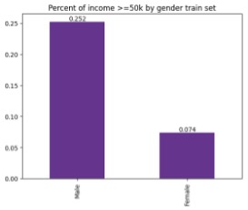
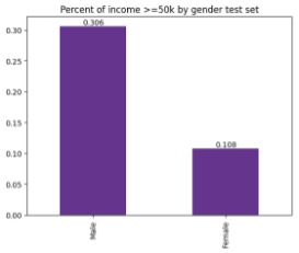
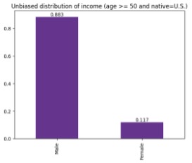
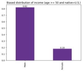
To mimic this shift in the data, for the purposes of our example, we split the dataset into training and production sets and artificially bias the labels in the latter towards more positive outcomes for the underrepresented group of females native to the U.S. over the age of 50.

Now, we first want to define the two worldviews of fairness² as defined in a recent Stanford lecture.

1. What you see is what you get: assumes that the training data is representative of the real world and that any biases in the data are reflective of the biases in society. A model making this assumption does not attempt to mitigate biases.
2. We are all equal: assumes that any differences in the outcomes of different groups are due to discrimination or bias in the data. A model making this assumption aims to make equal outcomes for all groups.

Therefore, fairness metrics can vary depending on how strict they are at ensuring fairness. Below we define the following which go from less strict to stricter and that we will use for our example:

• • Disparate Impact: Compares the percentage of positive outcomes for a protected group to the percentage of positive outcomes for an unprotected group. A value of 1 indicates no disparity, values greater than 1 indicate that the protected group is favored and values less than 1 indicate that the protected group is disfavored. Statistical differences between training and production sets may mean that the model has learned biased patterns for positive predictions on the training set that do not hold in the testing set
  • Equalized Odds: It ensures that the false positive and false negative rates are similar across all protected groups. A model is considered to have equalized odds if the false positive and false negative rates are similar for all protected groups. Statistical differences between training and production sets may mean there exist new biases present on the testing set which are significantly changing the false positive rate and/or false negative rates for the protected group (like an increase or decrease in the positive labels for that group)
  • Demographic parity: A model is considered to have statistical parity if the proportion of positive predictions is approximately the same for all protected groups. This is a strict measure of fairness whose goal is to ensure that the model’s predicted outcomes are statistically independent of the protected attribute. Statistical differences between training and production sets may mean that groups in the model’s predictions (or the new data) are being treated differently.

VIANOPS provides an easy-to-use API to monitor and evaluate any model’s fairness performance over time. As we will show, it can be tailored to the specific protected groups by creating and specifying them in segments of data and then retrieving their metrics.
After initializing our custom variables, our example notebook is divided into 3 main steps:

1. Creation of segments for protected and non-protected groups
2. Getting the performance metrics
3. Computation of fairness metrics

1. Creation of segments for protected and non-protected groups

We want to first define the segments in our data and protected and non-protected groups. In this example, the main group we are monitoring is that of females originally from the United States and over 50 years of age. We also add the segment for Black females to check whether it is also being affected by this drift and compute the fairness metrics on it. Thus, we define the following 6 segments:

Figure 3: (Below) Segment dictionary. ‘p’ and ‘np’ represent the protected and non-protected groups.

In the above dictionary we have the following inputs:

• • n_days: these are the number of days that we want to calculate the fairness metrics for both training and production sets. For statistical comparison, both sets must have the same number of days, in this case 30 where the first N days represent the training set and the next N days the production set.
  • filter: this is the feature and value of our main group or sensitive feature, in this example ‘gender=1’ represents the female population,
  • eval_features: we will define here the features we want to evaluate for fairness in conjunction with their protected and non-protected groups. For simplicity we have preprocessed those groups in the data to be 1 for protected and 0 for the rest.

After defining our segments, the post_segments() function will take care of registering them to the platform through our API.

 
2. Getting the performance metrics

Now, to retrieve our performance metrics over the set of 60 days of data, we call the function create_inference_mapping_preprocessing_for_mp_job() where we pass the start and end dates that we want to process, in this example, since we have the first 30 days as the training data and the next 30 as production, our start date is that of the first day of training and the end date that of production. Finally, we submit the job with submit_model_performance_job(). This function takes care of computing our performance metrics based on the segments of data we defined above and storing them appropriately in database.

 
3. Computation of fairness metrics

Finally, once the model performance job is completed, we are ready to retrieve the data from the model performance table. For this, we select them by model name and segment id as shown in the ‘Getting performance and fairness metrics’ section in the notebook. That will populate the segments_dict object with the responses from the dataset.

Now we can preprocess the data with get_fairness_metrics_dict() which will return a dictionary containing the disparate impact, demographic parity and equalized odds metrics each calculated per every day and feature (shown in Figure 5). Finally, we can perform our assessment of significant differences between training and production sets.

Figure 5: (Below) Demographic parity, disparate impact and equalized odds plots for the selected segments.

Figure 6: (Below) Statistical difference assessment between training and production sets for the equalized odds (EO), demographic parity (DP) and disparate impact (DI) fairness metrics and segments. Left: p-values for unbiased distribution, right: p-values for biased distribution. Bars below the dotted line represent significant changes for the particular metric and segment.

VIANOPS has thus aided us to detect and be aware that there has been a significant shift in the bias within the production data for said features and we can now take the appropriate actions to address them.

We have shown the importance of regularly monitoring your model’s performance using fairness metrics such as demographic parity, equalized odds and disparate impact to identify and flag biases early on. By means of fairness metrics, we can measure the imbalances on positive predictions between minority and majority groups from the beginning of our training and ensure that our models are updated so that we can take actions to ensure fairness. By doing so, we can take corrective actions such as augmenting the dataset with instances from underrepresented groups, balancing the training by oversampling from the minority class or undersampling from majority groups. This way we can avoid perpetuating bias ensuring equitable outcomes for all groups. VIANOPS enables organizations to monitor models for bias but also to do so in a highly scalable manner..

We’ve now made VIANOPS available free, for anyone to try. Try it out and let us know your feedback.

¹Becker & Kohavi. (1996). Adult. UCI Machine Learning Repository. https://doi.org/10.24432/C5XW20.

²Notions of fairness extracted from https://web.stanford.edu/class/cs329t/